Quick start
This notebook shows how to use osculari to conduct psychophysics on deep neural networks. We learn:
Extract features from an intermediate layer of the
ResNetnetwork.To train a two-alternative-forced-choice (2AFC) linear probe on the frozen pretrained network.
Evaluate the network’s sensitivity using the staircase procedure.
In this example, we are interested in evaluating the contrast sensitivity function (CSF) of deep neural networks.
![]()
If you are running this notebook on Google Colab, install osculari by uncommenting and executing the cell below.
# !pip install osculari
# importing required packages
import osculari

import numpy as np
from matplotlib import pyplot as plt
import torch
Pretrained features
Let’s create a linear classifier on top of the extracted features from a pretrained network to
perform a binary classification task (i.e., 2AFC – two-alternative-force-choice). This is easily
achieved by calling the paradigm_2afc_merge_concatenate from the osculari.models module.
architecture = 'resnet50'        # network's architecture
weights = 'resnet50'             # the pretrained weights
img_size = 224                   # network's input size
layer = 'block0'                 # the readout layer
pooling = None                   # whether reduce the spatial resolution of features by pooling
readout_kwargs = {               # parameters for extracting features from the pretrained network
    'architecture': architecture,
    'weights': weights,
    'layers': layer,
    'img_size': img_size,
    'pooling': pooling
}
net_2afc = osculari.models.paradigm_2afc_merge_concatenate(**readout_kwargs)
Dataset
The osculari.datasets module provides datasets that are generated randomly on the fly with
flexible properties that can be dynamically changed based on the experiment of interest.
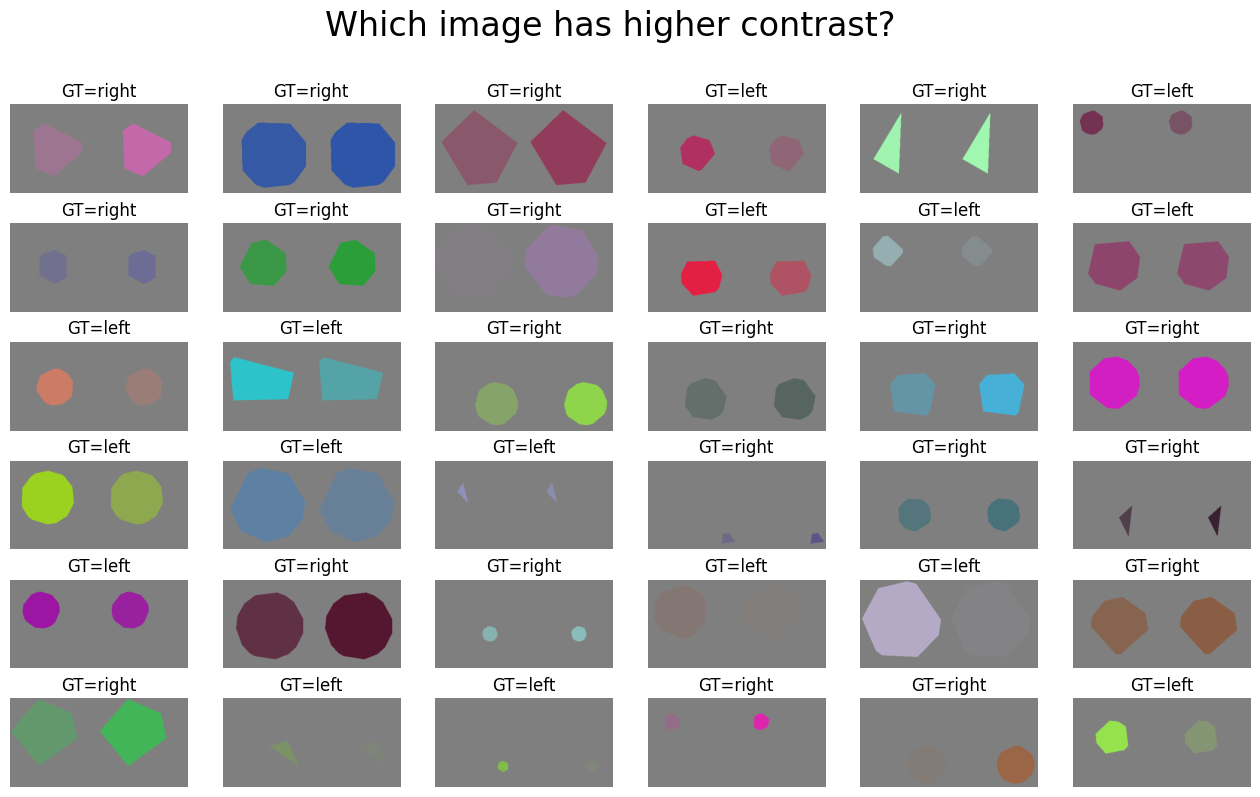
In this example, we use the ShapeAppearanceDataset class to create two images with different
levels of contrast. To do so, we pass the contrast_fun as the merging function that takes
care of experiment-dependent appearance settings. Other experiments can use the same template
and only implement a new merging function.
def contrast_fun(fgs, bgs):
    """
    Merging the foreground (fgs) and background (bgs) images. The ground truth is the
    image with a higher level of contrast.
    """
    num_imgs = len(fgs)
    contrast0, contrast1 = np.random.uniform(0.04, 1, 2)
    gt = 0 if contrast0 > contrast1 else 1
    contrasts = [contrast0, contrast1]
    colour = [np.random.randint(0, 256) for _ in range(3)]
    imgs = []
    for i in range(num_imgs):
        img = bgs[i].copy()
        for c in range(3):
            chn = img[..., c]
            chn[fgs[i]] = colour[c] / 255
            img[..., c] = chn
        img = (1 - contrasts[i]) / 2.0 + np.multiply(img, contrasts[i])
        imgs.append(img)
    return imgs, gt
num_samples = 1000               # the number of random samples generated in the dataset
num_imgs = net_2afc.input_nodes  # the number of images in each sample
background = 128                 # the background type
dataset = osculari.datasets.geometrical_shapes.ShapeAppearanceDataset(
    num_samples, num_imgs, img_size, background, contrast_fun,
    unique_bg=True, transform=net_2afc.preprocess_transform()
)
# visualising a few samples from our dataset
fig = plt.figure(figsize=(16, 9))
fig.suptitle('Which image has higher contrast?', fontsize=24)
for i in range(36):
    # one sample from dataset
    sample = dataset.__getitem__(i)
    ax = fig.add_subplot(6, 6, i+1)
    # concatenating  the images for visualisation
    disp_img = np.concatenate([sample[0], sample[1]], axis=2)
    # convering torch images to numpy
    disp_img = disp_img.transpose(1, 2, 0)
    disp_img = disp_img * net_2afc.normalise_mean_std[1] + net_2afc.normalise_mean_std[0]
    ax.imshow(disp_img)
    ax.set_title('GT=%s' % ('left' if sample[2] == 0 else 'right'))
    ax.axis('off')
Linear Probe
The osculari.paradigms module implements a set of psychophysical paradigms. The train_linear_probe
function trains the network on a dataset following the paradigm passed to the function.
# experiment-dependent function to process an epoch of data
epoch_fun = osculari.paradigms.forced_choice.epoch_loop
# calling the generic train_linear_probe function
training_log = osculari.paradigms.paradigm_utils.train_linear_probe(
    net_2afc, dataset, epoch_fun, './osculari_test/'
)
[000] accuracy=0.629 loss=147751.149
[001] accuracy=0.654 loss=275464.128
[002] accuracy=0.628 loss=369011.674
[003] accuracy=0.727 loss=178726.005
[004] accuracy=0.659 loss=394008.253
[005] accuracy=0.814 loss=73967.540
[006] accuracy=0.841 loss=60744.452
[007] accuracy=0.846 loss=54002.296
[008] accuracy=0.884 loss=32547.235
[009] accuracy=0.883 loss=42578.707
Psychophysical experiment
The osculari.paradigms module also implements a set of psychophysical experiments similar to the
experiments conducted with human participants. In this example, we use the staircase function
to gradually measure the network’s sensitivity.
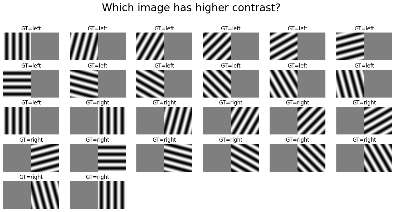
class ContrastGratingsDataset(osculari.datasets.gratings.GratingsDataset):
    """Returning two gratings, one uniform gray and another with sinusoidal gratings."""

    def __init__(self, contrasts, img_size, spatial_frequency, **kwargs):
        super(ContrastGratingsDataset, self).__init__(
            img_size=img_size, spatial_frequencies=[spatial_frequency], **kwargs
        )
        self.contrasts = contrasts


    def __getitem__(self, idx):
        stimuli0 = self.make_grating(idx, self.contrasts[0])
        stimuli1 = self.make_grating(idx, self.contrasts[1])
        if self.transform:
            stimuli0 = self.transform(stimuli0).float()
            stimuli1 = self.transform(stimuli1).float()
        gt = np.argmax(self.contrasts)
        return stimuli0, stimuli1, gt
def dataset_fun(contrast_level, spatial_frequency, transform, img_size):
    dataset_kwargs = {
        'img_size': img_size,
        'spatial_frequency': spatial_frequency,
        'gaussian_sigma': None,
        'transform': transform
    }
    test_dataset = torch.utils.data.ConcatDataset([
        ContrastGratingsDataset([contrast_level, 0], **dataset_kwargs),
        ContrastGratingsDataset([0, contrast_level], **dataset_kwargs)
    ])
    return test_dataset, test_dataset.__len__(), 0.749
# visualising all samples for test set with spatial frequency equals 4
fig = plt.figure(figsize=(16, 9))
fig.suptitle('Which image has higher contrast?', fontsize=24)
test_dataset, _, _ = dataset_fun(1, 4, net_2afc.preprocess_transform(), img_size)
for i in range(test_dataset.__len__()):
    # one sample from dataset
    sample = test_dataset.__getitem__(i)
    ax = fig.add_subplot(6, 6, i+1)
    # concatenating  the images for visualisation
    disp_img = np.concatenate([sample[0], sample[1]], axis=2)
    # convering torch images to numpy
    disp_img = disp_img.transpose(1, 2, 0)
    disp_img = disp_img * net_2afc.normalise_mean_std[1] + net_2afc.normalise_mean_std[0]
    ax.imshow(np.maximum(np.minimum(disp_img, 1), 0))
    ax.set_title('GT=%s' % ('left' if sample[2] == 0 else 'right'))
    ax.axis('off')
# experiment-dependent function to test an epoch of data
test_epoch_fun = osculari.paradigms.forced_choice.test_dataset

sfs = [i for i in range(1, img_size // 2 + 1) if img_size % i == 0]
csf = []
# looping through all spatial frequencies
for sf in sfs:
    db_fun = lambda contrast: dataset_fun(contrast, sf, net_2afc.preprocess_transform(), img_size)
    # calling the staircase procedure for current spatial frequency
    test_log = osculari.paradigms.staircase(net_2afc, test_epoch_fun, db_fun, low_val=0, high_val=1)
    # the first column of the last row in test_log is the contrast at threshold
    csf.append(test_log[-1, 0])
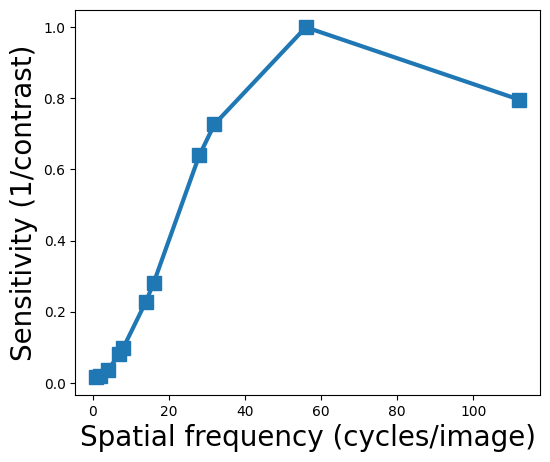
We have obtained the CSF of block0 of ResNet50 which can be directly compared to human data
to investigate whether they are similar or not.
# let's visualise the obtained CSF
fig = plt.figure(figsize=(6, 5))
ax = fig.add_subplot(1, 1, 1,)
sensitivity = 1 / np.array(csf)
sensitivity /= sensitivity.max()
ax.plot(np.array(sfs), sensitivity, '-s', markersize=10, linewidth=3)
ax.set_xlabel('Spatial frequency (cycles/image)', fontsize=20)
ax.set_ylabel('Sensitivity (1/contrast)', fontsize=20)
plt.show()