Odd-one-out paradigm

This notebook shows how to use osculari to perform the odd-one-out paradigm. The linear probe’s output is the index of the odd image among three or more images. The flexibility of this paradigm makes it powerful to conduct conflicting-cues psychophysical experiments.

If you are running this notebook on Google Colab, install osculari by uncommenting and executing the cell below.

# !pip install osculari

# importing required packages
from osculari import models, datasets, paradigms

import numpy as np
from matplotlib import pyplot as plt
import torch

Pretrained features

Let’s create a linear classifier on top of the extracted features from a pretrained network to perform a 4AFC odd-one-out (OOO) task (i.e., which image out of four options is the “odd” one). The models.paradigm_ooo_merge_difference() function implements a generic odd-one-paradigms among any number of images. In this example, we use 4AFC (i.e., among four images) by passing the input_nodes=4 argument.

architecture = 'vit_b_32'        # network's architecture
weights = 'vit_b_32'             # the pretrained weights
img_size = 224                   # network's input size
layer = 'block7'                 # the readout layer
pooling = None                   # whether reduce the spatial resolution of features by pooling
readout_kwargs = {               # parameters for extracting features from the pretrained network
    'architecture': architecture, 
    'weights': weights,
    'layers': layer,
    'img_size': img_size,
    'pooling': pooling 
}
net_odd4 = models.readout.paradigm_ooo_merge_difference(input_nodes=4, **readout_kwargs)

Dataset

The osculari.datasets module provides datasets that are generated randomly on the fly with flexible properties that can be dynamically changed based on the experiment of interest. In this example, we use the ShapeAppearanceDataset class to create four images: three of them having an identical physical colour and one with a different colour. To do so, we pass the odd_one_colour as the merging function that handles experiment-dependent appearance settings. Other experiments can use the same template and only implement a new merging function.

def odd_one_colour(fgs, bgs):
    """
    Merging foreground masks (fgs) into background images (bgs). The ground truth is the
    index of the odd image (with a different colour).
    """
    num_imgs = len(fgs)
    gt = np.random.randint(0, num_imgs)
    colour0 = datasets.dataset_utils.random_colour()
    colour1 = datasets.dataset_utils.random_colour()
    colours = [colour0 if g == gt else colour1 for g in range(num_imgs)]
    imgs = []
    for i in range(num_imgs):
        img = bgs[i].copy()
        for c in range(3):
            chn = img[..., c]
            chn[fgs[i]] = colours[i][c] / 255
            img[..., c] = chn
        imgs.append(img)
    return imgs, gt

num_samples = 1000               # the number of random samples generated in the dataset
num_imgs = net_odd4.input_nodes  # the number of images in each sample
background = 128                 # the background type
merge_fg_bg = odd_one_colour     # the function in charge of merging foreground and background
dataset = datasets.ShapeAppearanceDataset(
    num_samples, num_imgs, img_size, background, merge_fg_bg,
    unique_bg=True, transform=net_odd4.preprocess_transform()
)

def visualise_dataset(dataset, net_odd):
    """A helper function to visualise dataset images."""
    # visualising a few samples from our dataset
    fig = plt.figure(figsize=(16, 6))
    fig.suptitle('Which image is the odd one?', fontsize=24)
    for i in range(36):
        # one sample from dataset
        sample = dataset.__getitem__(i)
        ax = fig.add_subplot(6, 6, i+1)
        # concatenating  the images for visualisatiaon
        disp_img = np.concatenate(sample[:-1], axis=2)
        # convering torch images to numpy
        disp_img = disp_img.transpose(1, 2, 0)
        # inverting the normalisation
        disp_img = disp_img * net_odd.normalise_mean_std[1] + net_odd.normalise_mean_std[0]
        # ensuring the images are in the range of 0 to 1
        disp_img = np.maximum(np.minimum(disp_img, 1), 0)
        ax.imshow(disp_img)
        ax.set_title('GT=%d' % sample[-1])
        ax.axis('off')

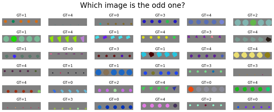
Let’s visualise a few examples from our dataset to better understand the task of 4AFC OOO. We can see that in each sample, three images have an identical colour while one image has a different colour. In this example, the shapes are identical for each sample. This can easily be changed, by passing the unique_fg_shape=False argument. Please look at the usage page.

visualise_dataset(dataset, net_odd4)

Linear Probe

The osculari.paradigms module implements a set of psychophysical paradigms. The train_linear_probe function trains the network on a dataset following the paradigm passed to the function.

These set of lines are identical to the 2AFC task we looked at in the quick start notebook, showing that for many paradigms you only have to implement the dataloader/dataset component of your experiment.

The network reaches perfect accuracy in only 3 epochs. The simplicity of the task for linear probes are often intentional, as their purpose is to open a communication channel to pretrained network for follow-up psychophysical experiments.

# the output directory
out_dir = './oddoneout_4afc/'
# experiment-dependent function to process an epoch of data
epoch_fun = paradigms.forced_choice.epoch_loop
# calling the generic train_linear_probe function
training_log = paradigms.paradigm_utils.train_linear_probe(
    net_odd4, dataset, epoch_fun, out_dir, epochs=3
)

[000] accuracy=0.988 loss=0.022
[001] accuracy=1.000 loss=0.000
[002] accuracy=1.000 loss=0.000

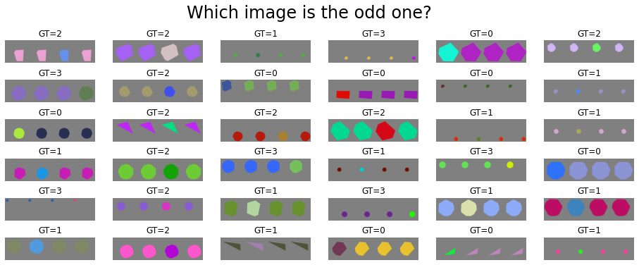
3AFC

To change our paradigm from 4AFC to 3AFC requries only changing one parameter in the network: input_nodes=3. We do not need to change anythign else, the dataset authomatically obtained the input_nodes from network. The training procedure (e.g., loss function) also handles the input_nodes directly from the network.

# network
net_odd3 = models.readout.paradigm_ooo_merge_difference(input_nodes=3, **readout_kwargs)
# dataset
dataset = datasets.ShapeAppearanceDataset(
    num_samples, net_odd3.input_nodes, img_size, background, merge_fg_bg,
    unique_bg=True, transform=net_odd3.preprocess_transform()
)
visualise_dataset(dataset, net_odd3)

# the output directory
out_dir = './oddoneout_3afc/'
# experiment-dependent function to process an epoch of data
epoch_fun = paradigms.forced_choice.epoch_loop
# calling the generic train_linear_probe function
training_log = paradigms.paradigm_utils.train_linear_probe(
    net_odd3, dataset, epoch_fun, out_dir, epochs=3
)

[000] accuracy=0.993 loss=0.018
[001] accuracy=1.000 loss=0.000
[002] accuracy=1.000 loss=0.000

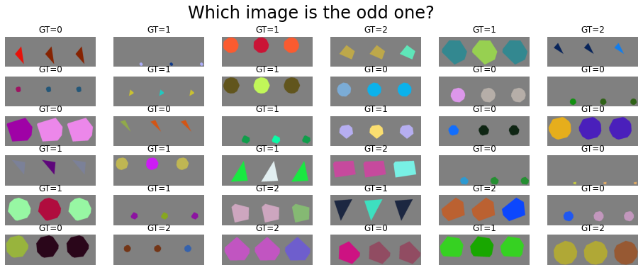
5AFC

We can also easily increase the numebr of images in the odd-one-out task. Having more images allows for a larger combination of conflicting features, which is outside the scope of this tutorial.

# network
net_odd5 = models.readout.paradigm_ooo_merge_difference(input_nodes=5, **readout_kwargs)
# dataset
dataset = datasets.ShapeAppearanceDataset(
    num_samples, net_odd5.input_nodes, img_size, background, merge_fg_bg,
    unique_bg=True, transform=net_odd5.preprocess_transform()
)
visualise_dataset(dataset, net_odd5)

# the output directory
out_dir = './oddoneout_5afc/'
# experiment-dependent function to process an epoch of data
epoch_fun = paradigms.forced_choice.epoch_loop
# calling the generic train_linear_probe function
training_log = paradigms.paradigm_utils.train_linear_probe(
    net_odd5, dataset, epoch_fun, out_dir, epochs=3
)

[000] accuracy=0.986 loss=0.026
[001] accuracy=0.999 loss=0.002
[002] accuracy=1.000 loss=0.000