Usage

This notebook demonstrates how to use the osculari package.

The osculari package is organized into three main modules:

• models: Used for reading pretrained networks and adding linear layers on top of them.

• datasets: Used to create datasets and dataloaders for training and testing linear probes.

• paradigms: Used to implement psychophysical paradigms for experimenting with deep networks.

If you are running this notebook on Google Colab, install osculari by uncommenting and executing the cell below.

# !pip install osculari

# importing required packages
import osculari
from osculari import models, datasets, paradigms

import numpy as np
import requests
from matplotlib import pyplot as plt
from PIL import Image as pil_image
import torch
import torchvision.transforms as torch_transforms

osculari.models

Supported models

To check which models are supported by osculari, call the available_models() function, which returns a dictionary corresponding to different datasets/environments:

• imagenet

• segmentation

• taskonomy

• clip Each item in the dictionary contains a list of supported pretrained networks.

Calling the available_models(flatten=True) returns a list of all supported models without splitting them into datasets/environments.

models.available_models()

{'imagenet': ['alexnet',
  'convnext_base',
  'convnext_large',
  'convnext_small',
  'convnext_tiny',
  'densenet121',
  'densenet161',
  'densenet169',
  'densenet201',
  'efficientnet_b0',
  'efficientnet_b1',
  'efficientnet_b2',
  'efficientnet_b3',
  'efficientnet_b4',
  'efficientnet_b5',
  'efficientnet_b6',
  'efficientnet_b7',
  'efficientnet_v2_l',
  'efficientnet_v2_m',
  'efficientnet_v2_s',
  'googlenet',
  'inception_v3',
  'maxvit_t',
  'mnasnet0_5',
  'mnasnet0_75',
  'mnasnet1_0',
  'mnasnet1_3',
  'mobilenet_v2',
  'mobilenet_v3_large',
  'mobilenet_v3_small',
  'regnet_x_16gf',
  'regnet_x_1_6gf',
  'regnet_x_32gf',
  'regnet_x_3_2gf',
  'regnet_x_400mf',
  'regnet_x_800mf',
  'regnet_x_8gf',
  'regnet_y_128gf',
  'regnet_y_16gf',
  'regnet_y_1_6gf',
  'regnet_y_32gf',
  'regnet_y_3_2gf',
  'regnet_y_400mf',
  'regnet_y_800mf',
  'regnet_y_8gf',
  'resnet101',
  'resnet152',
  'resnet18',
  'resnet34',
  'resnet50',
  'resnext101_32x8d',
  'resnext101_64x4d',
  'resnext50_32x4d',
  'shufflenet_v2_x0_5',
  'shufflenet_v2_x1_0',
  'shufflenet_v2_x1_5',
  'shufflenet_v2_x2_0',
  'squeezenet1_0',
  'squeezenet1_1',
  'swin_b',
  'swin_s',
  'swin_t',
  'swin_v2_b',
  'swin_v2_s',
  'swin_v2_t',
  'vgg11',
  'vgg11_bn',
  'vgg13',
  'vgg13_bn',
  'vgg16',
  'vgg16_bn',
  'vgg19',
  'vgg19_bn',
  'vit_b_16',
  'vit_b_32',
  'vit_h_14',
  'vit_l_16',
  'vit_l_32',
  'wide_resnet101_2',
  'wide_resnet50_2'],
 'segmentation': ['deeplabv3_mobilenet_v3_large',
  'deeplabv3_resnet101',
  'deeplabv3_resnet50',
  'fcn_resnet101',
  'fcn_resnet50'],
 'taskonomy': ['taskonomy_autoencoding',
  'taskonomy_class_object',
  'taskonomy_class_scene',
  'taskonomy_colorization',
  'taskonomy_curvature',
  'taskonomy_denoising',
  'taskonomy_depth_euclidean',
  'taskonomy_depth_zbuffer',
  'taskonomy_edge_occlusion',
  'taskonomy_edge_texture',
  'taskonomy_egomotion',
  'taskonomy_fixated_pose',
  'taskonomy_inpainting',
  'taskonomy_jigsaw',
  'taskonomy_keypoints2d',
  'taskonomy_keypoints3d',
  'taskonomy_nonfixated_pose',
  'taskonomy_normal',
  'taskonomy_point_matching',
  'taskonomy_reshading',
  'taskonomy_room_layout',
  'taskonomy_segment_semantic',
  'taskonomy_segment_unsup25d',
  'taskonomy_segment_unsup2d',
  'taskonomy_vanishing_point'],
 'clip': ['clip_RN50',
  'clip_RN101',
  'clip_RN50x4',
  'clip_RN50x16',
  'clip_RN50x64',
  'clip_ViT-B/32',
  'clip_ViT-B/16',
  'clip_ViT-L/14',
  'clip_ViT-L/14@336px']}

Pretrained networks

The main entry to pretrained networks is the models.readout submodule, which supports several functionalities.

Feature extraction

To extract features from a pretrained network at a specific layer, call the FeatureExtractor class, passing the following arguments:

• architecture is the network’s architecture you want to load (e.g. resnet50 or vit_b_32). It should be one of the items from the available models we mentioned above.

• weights defines the pretrained weights. It can be one of the following formats:

  • Path to a local file.

  • Downloadable URL of the pretrained weights.

  • A string corresponding to the available weight, for instance, PyTorch resnet50 supports one of the following strings: [”DEFAULT”, “IMAGENET1K_V1”, “IMAGENET1K_V2”].

  • The same name as architecture, which loads the network’s default weights.

• layers determines the read-out (cut-off) layer(s). Which layers are available for each network can be obtained by calling the models.available_layers() function.

In this example, we extract features from the first block of ResNet50, using the default weights.

architecture = 'resnet50'        # network's architecture
weights = 'resnet50'             # the pretrained weights
layer = 'block0'                 # the readout layer
readout_kwargs = {               # parameters for extracting features from the pretrained network
    'architecture': architecture, 
    'weights': weights,
    'layers': layer,
}
feature_extractor = models.FeatureExtractor(**readout_kwargs)
print(feature_extractor)

FeatureExtractor(
  (backbone): Sequential(
    (0): Conv2d(3, 64, kernel_size=(7, 7), stride=(2, 2), padding=(3, 3), bias=False)
    (1): BatchNorm2d(64, eps=1e-05, momentum=0.1, affine=True, track_running_stats=True)
    (2): ReLU(inplace=True)
    (3): MaxPool2d(kernel_size=3, stride=2, padding=1, dilation=1, ceil_mode=False)
  )
)

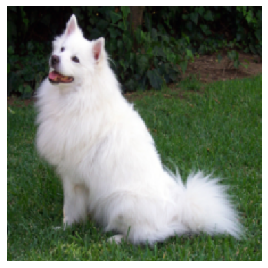
Let’s open an image and test our feature_extractor. We should convert the image into a torch tensor. Each pretrained network has its own mean and std for normalisation. These values are available from the class variable normalise_mean_std.

# reading an image
url = 'https://github.com/pytorch/hub/raw/master/images/dog.jpg'
input_img = pil_image.open(requests.get(url, stream=True).raw)

img_size = 224
mean, std = feature_extractor.normalise_mean_std
# converting it to torch tensor
transforsm = torch_transforms.Compose([
    torch_transforms.Resize((img_size, img_size)),
    torch_transforms.ToTensor(),
    torch_transforms.Normalize(mean=mean, std=std)
])
torch_img = torch.stack([transforsm(input_img)])
print('Shape of the input image:', torch_img.shape)

# visualising the image that will be input to the network
img_vis = torch_img.numpy().squeeze().transpose(1, 2, 0) * std + mean
img_vis = np.maximum(np.minimum(img_vis, 1), 0)
plt.imshow(img_vis)
plt.axis('off')
plt.show()

Shape of the input image: torch.Size([1, 3, 224, 224])

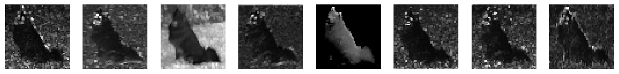
We can now extract features for our image. Note that feature_extractor is like any other torch.nn.Module and is callable. In this exampple, we input the network with one image, but multiple images can also be input.

# extragin the features
features = feature_extractor(torch_img)
print('Shape of the extracted features:', features.shape)

Shape of the extracetd features: torch.Size([1, 64, 56, 56])

# visualising 8 of the extracted features
fig = plt.figure(figsize=(16, 4))
for i in range(8):
    ax = fig.add_subplot(1, 8, i+1)
    ax.matshow(features[0, i].detach().numpy(), cmap='gray')
    ax.axis('off')

Pooling

From the feature extractor example, we can observe that the dimensionality of the extracted features might be too large–a vector of \(200704\) elements (\(64 \times 56 \times 56\))– to input directly to a linear classifier. It might be beneficial to reduce this using pooling operations that do not have extra parameters to learn. We can achieve this by passing the 'pooling' parameter.

In this example, we pass 'pooling': 'avg_2_2' (i.e., adaptive average pooling with a \(2 \times 2\) output size. We can see that the extracted features are only \(256\) elements (\(64 \times 2 \times 2\)).

architecture = 'resnet50'        # network's architecture
weights = 'resnet50'             # the pretrained weights
img_size = 224                   # network's input size
layer = 'block0'                 # the readout layer
pooling = 'avg_2_2'              # whether reduce the spatial resolution of features by pooling
readout_kwargs = {               # parameters for extracting features from the pretrained network
    'architecture': architecture, 
    'weights': weights,
    'layers': layer,
    'pooling': pooling 
}
feature_extractor = models.FeatureExtractor(**readout_kwargs)

# extracting features
features = feature_extractor(torch_img)
print('Shape of the extracted features with pooling:', features.shape)

Shape of the extracted features with pooling: torch.Size([1, 1, 64, 2, 2])

From the print above you can note that the output contains five dimensions:

1. batch size, in this example 1.

2. Corresponding to the number of pooling operations, which we explain below.

3. Number of kernels, in this example 64.

4. Width of spatial resolution.

5. Height of spatial resolution.

Currently, we support two pooling operations: AdaptiveAvgPool2d and AdaptiveMaxPool2d. The 'pooling' parameter can be one of the following formats:

• avg_x_y: applying an adaptive average pooling with a \(x \times y\) output size,

• max_x_y: applying an adaptive max pooling,

• maxavg_x_y or avgmax_x_y: applying both pooling operations; under this scenario the output’s second dimension will be 2 always in this order: average pooling is always first.

Linear probing

Linear probing is a powerful and flexible technique for interpreting intermediate representation in deep networks. This consists of adding a linear layer on top of the features extracted from a frozen pretrained network. This can be easily archived by inheriting the readout.ProbeNet class.

For instance, let’s say we want to perform a 2AFC task, we can implement Classifier2AFC class:

• input_nodes=2 specifies that the number of input images passed to the linear classifier is two.

• num_classes=2 denotes that the linear classifier outputs two numbers.

• We should implement the forward function. In this example, we extract features from two inputs and concatenate them into one vector, which is input to the probe layer.

Other custom paradigms are easily achieved by changing the input_nodes, num_classes and forward function.

class Classifier2AFC(models.readout.ProbeNet):
    def __init__(self, **kwargs) -> None:
        super(Classifier2AFC, self).__init__(input_nodes=2, num_classes=2, **kwargs)

    def forward(self, x0, x1):
        x0 = self.do_features(x0)
        x1 = self.do_features(x1)
        x = torch.cat([x0, x1], dim=1)
        return self.do_probe_layer(x)

Let’s make an instance of the Classifier2AFC we just created.

architecture = 'resnet50'        # network's architecture
weights = 'resnet50'             # the pretrained weights
img_size = 224                   # network's input size
layer = 'block0'                 # the readout layer
pooling = None                   # whether reduce the spatial resolution of features by pooling
readout_kwargs = {               # parameters for extracting features from the pretrained network
    'architecture': architecture, 
    'weights': weights,
    'layers': layer,
    'img_size': img_size,
    'pooling': pooling 
}
net_2afc = Classifier2AFC(**readout_kwargs)
print(net_2afc)

Classifier2AFC(
  (backbone): Sequential(
    (0): Conv2d(3, 64, kernel_size=(7, 7), stride=(2, 2), padding=(3, 3), bias=False)
    (1): BatchNorm2d(64, eps=1e-05, momentum=0.1, affine=True, track_running_stats=True)
    (2): ReLU(inplace=True)
    (3): MaxPool2d(kernel_size=3, stride=2, padding=1, dilation=1, ceil_mode=False)
  )
  (fc): Linear(in_features=401408, out_features=2, bias=True)
)

After printing the net_2afc, we can see that the Classifier2AFC network contains two nodes:

• backbone

• fc

corresponding to the pretrained network and linear classifier, respectively.

Now, we can call our net_2afc with two images.

Of course, the linear layer should be trained on some tasks to obtain meaningful results. Please check the examples page of our documentation.

output = net_2afc(torch_img, torch_img)
print("Shape of the Classifier2AFC output:", output.shape)

Shape of the Classifier2AFC output: torch.Size([1, 2])

Predefined paradigms

Common paradigms like 2AFC are already implemented. For instance, using the models.paradigm_2afc_merge_concatenate function results in a similar network we implemented above. Check the models documentation to see all paradigms already implemented.

architecture = 'resnet50'        # network's architecture
weights = 'resnet50'             # the pretrained weights
img_size = 224                   # network's input size
layer = 'block0'                 # the readout layer
pooling = None                   # whether reduce the spatial resolution of features by pooling
readout_kwargs = {               # parameters for extracting features from the pretrained network
    'architecture': architecture, 
    'weights': weights,
    'layers': layer,
    'img_size': img_size,
    'pooling': pooling 
}
net_2afc = models.paradigm_2afc_merge_concatenate(**readout_kwargs)
print(net_2afc)

Classifier2AFC(
  (backbone): Sequential(
    (0): Conv2d(3, 64, kernel_size=(7, 7), stride=(2, 2), padding=(3, 3), bias=False)
    (1): BatchNorm2d(64, eps=1e-05, momentum=0.1, affine=True, track_running_stats=True)
    (2): ReLU(inplace=True)
    (3): MaxPool2d(kernel_size=3, stride=2, padding=1, dilation=1, ceil_mode=False)
  )
  (fc): Linear(in_features=401408, out_features=2, bias=True)
)

osculari.datasets

The linear probe layer must be trained on some data to obtain meaningful results. The training dataset highly depends on the feature one is interested in studying. Nevertheless, the datasets module implements a few generic datasets that are helpful in many scenarios.

ShapeAppearanceDataset

The datasets.ShapeAppearanceDataset implements a generic foreground-background images allowing an easy interface to manipulate foreground appearance and merge it into the background. To achieve this, pass a merge_fg_bg function to this dataset.

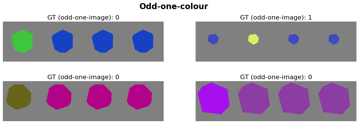
Let’s make an example, where we create four images for an odd-one-out task based on the object’s colour.

def odd_one_colour(fgs, bgs):
    """Merging foreground masks (fgs) into background images (bgs)."""
    num_imgs = len(fgs)
    gt = np.random.randint(0, num_imgs)
    colour0 = datasets.dataset_utils.random_colour()
    colour1 = datasets.dataset_utils.random_colour()
    colours = [colour0 if g == gt else colour1 for g in range(num_imgs)]
    imgs = []
    for i in range(num_imgs):
        img = bgs[i].copy()
        for c in range(3):
            chn = img[..., c]
            chn[fgs[i]] = colours[i][c] / 255
            img[..., c] = chn
        imgs.append(img)
    return imgs, gt

num_samples = 1000               # the number of random samples generated in the dataset
num_imgs = 4                     # the number of images in each sample
background = 128                 # the background type
merge_fg_bg = odd_one_colour     # the function in charge of merging foreground and background
dataset = datasets.ShapeAppearanceDataset(
    num_samples, num_imgs, img_size, background, merge_fg_bg,
)

The merge_fg_bg decides the output of __getitem__ function. In this example, we return four images and one ground-truth.

db_out = dataset.__getitem__(i)
print('Number of elements in dataset output:', len(db_out))
imgs = db_out[:-1]
gt = db_out[-1]
print('Images spatial resolution:', [el.shape for el in imgs])
print('Ground-truth:', gt)

Number of elements in dataset output: 5
Images spatial resolution: [(224, 224, 3), (224, 224, 3), (224, 224, 3), (224, 224, 3)]
Ground-truth: 1

Let’s get a few items from our dataset and visualise them:

def plot_dataset(dataset, num_sampels, title):
    fig = plt.figure(figsize=(16, num_sampels+1))
    fig.suptitle(title, fontsize=20, fontweight='bold')
    for i in range(num_sampels):
        db_out = dataset.__getitem__(i)
        imgs = db_out[:-1]
        ax = fig.add_subplot(num_sampels//2, 2, i+1)
        ax.set_title('GT (odd-one-image): %d' % db_out[-1], fontsize=16)  
        ax.imshow(np.concatenate(imgs, axis=1))
        ax.axis('off')

plot_dataset(dataset, 4, 'Odd-one-colour')

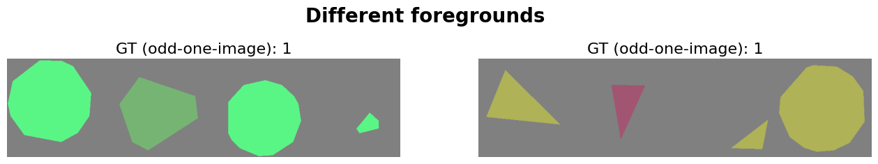
Several aspects of the ShapeAppearanceDataset can easily be modified including. Let’s look at a few example:

# making the foreground shapes different
dataset = osculari.datasets.ShapeAppearanceDataset(
    num_samples, num_imgs, img_size, background, merge_fg_bg,
    unique_fg_shape=False
)
plot_dataset(dataset, 2, 'Different foregrounds')

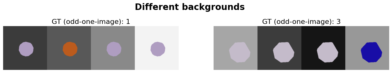
# making the foreground shapes different
dataset = datasets.ShapeAppearanceDataset(
    num_samples, num_imgs, img_size, merge_fg_bg=merge_fg_bg,
    background='uniform_achromatic', unique_bg=False
)
plot_dataset(dataset, 2, 'Different backgrounds')

osculari.paradigms

Similar to the training dataset of the linear probe layer, the procedure to train/test this layer is also task-dependent. Nevertheless, the paradigms module implements a few generic train/test routines that are useful in many scenarios.

Training

The paradigms.train_linear_probe function offers generic training for the linear layer.

The following arguments must be passed to this function:

• model: for instance the net_2afc we created above.

• dataset: for instance the `dataset we create above.

• epoch_loop: a callable function that processes an epoch of data. Several paradigms already implement such a function (e.g., paradigms.forced_choice.epoch_loop that handles any alternative-forced-choice task, such as 2AFC and 4AFC). Alternatively, you can implement a custom function yourself.

• out_dir: to save the checkpoints.

The following arguments are optional (a reasonable default exists for them):

• optimiser [default is SGD with \(lr=0.1\)].

• epochs [default is 10].

• scheduler [default is MultiStepLR at 50 and 80% of epochs].

The paradigms.train_linear_probe save the checkpoints and return the log values for all epochs (i.e., each epoch log is a Dict the output of the epoch_loop function).

Please check the examples page of our documentation that showcases a few notebooks using this function.

Psychophysics

Finally, once the linear probe is trained, we can conduct the psychophysical experiments with it to learn more about the internal representation of deep networks.

The paradigms module also implements a set of common psychophysical experiments similar to the experiments conducted with human participants. For instance, the paradigms.staircase function implements the staircase procedure to measure the sensitivity threshold by adjusting the value of the features we are interested in studying.

Please check the paradigms documentation to see all psychophysical paradigms already implemented.

Please check the examples page of our documentation that showcases a few notebooks using this function.